Revealing the Strategies Hidden in Variance

Variance and Golf Design (Part Two)

Introduction

This is the second part of a discussion about variance in golf. It started out as a long-form piece that involved a ton of programming for the visualizations. Now that the work is done, I’m breaking it up into three parts so it will be a bit more palatable. Here, though, remember that I’m trying to build up to something throughout the three-part series.

• Part one was about how hole design transforms uniform dispersion patterns into different probabilistic outputs.

• Part two is about visualizing variance: how we can show strategic tradeoffs by illustrating risk-adjusted strokes to hole.

• Part three will be about what we mean by “good shots” and “bad shots,” and will illustrate why the two different frameworks divide the golf community.

In part one, I outlined the idea that golf course features transform shot quality into result quality. We can think of this as taking the input randomness (the golfer’s dispersion pattern) and then converting that random distribution into a different distribution by the way the ball interacts with the golf course’s architectural features, hazards, etc. Strategic golf is the process by which the player tries to optimize that transformation by choosing to aim at a target that isn’t simply the closest point to the hole. This background is necessary for the next step of looking at the variance across an entire golf hole. Doing that requires us to add a third calculation: chaining the variance of different shots together.

Note: this is going to be a very technical article. While it’s not entirely necessary, if you’re new to the blog, I would recommend reading the very first post about my golf architecture visualizer as a prerequisite, because it describes the process of creating these visualizations.

What Overall Variance Looks Like

Map #1: Optimal Shot Standard Deviation

The most basic variance illustration I can produce is a heatmap of the standard deviation of the expected strokes to hole from every location on the map. We first have to calculate the optimal shot from every point on the course, but after that, this map highlights the parts of the hole where a good versus bad result on that shot will have an outsized impact on expected score.

#8 at Sharp Park

Let’s start with a very basic hole: #8 at Sharp Park is about as simple as it gets. It is a mostly flat and very short par three.

Standard deviation map of #8 at Sharp Park. The video above shows both the hole and how low-variance it is. Even a poor tee shot that misses the green still leaves this player with a realistic putt for par.

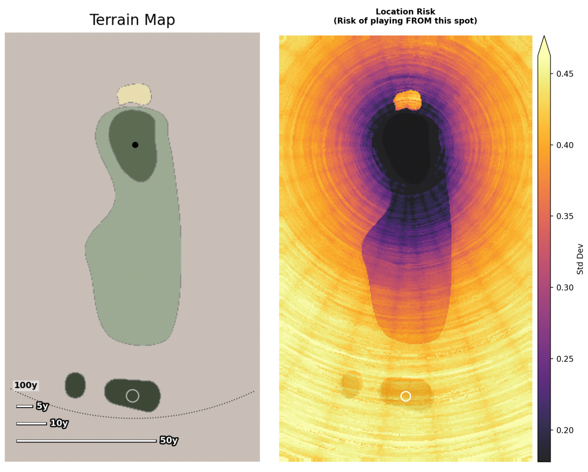
This map shows us the variance in expected strokes to hole from every position on the golf hole. If a pixel is purple, that means a shot from that position should result in similar expected strokes to hole. If the pixel is yellow, it means that we should expect some of the shots from that location to lead to low expected scores and other shots to lead to high expected scores.

The most obvious area with highly variable results is the (bright orange) bunker in the (purple) rough behind the green. Most chips from the rough will lead to a putt or two, but hitting from the sand can lead to wildly different results (both good and bad).

#8 at Sharp Park is extremely short and simple. The main impact on variance is distance. We see this reflected in the circular gradient that smoothly moves from low variance to higher variance.

#8 at Royal Troon

In contrast, if we want a high-variance hole, we should look at #8 at Troon: the Postage Stamp.

Standard deviation map of #8 at Royal Troon. The video above shows both the hole and how high-variance it is. Even great tee shots that barely miss the cup can roll off and leave players in a bunker.

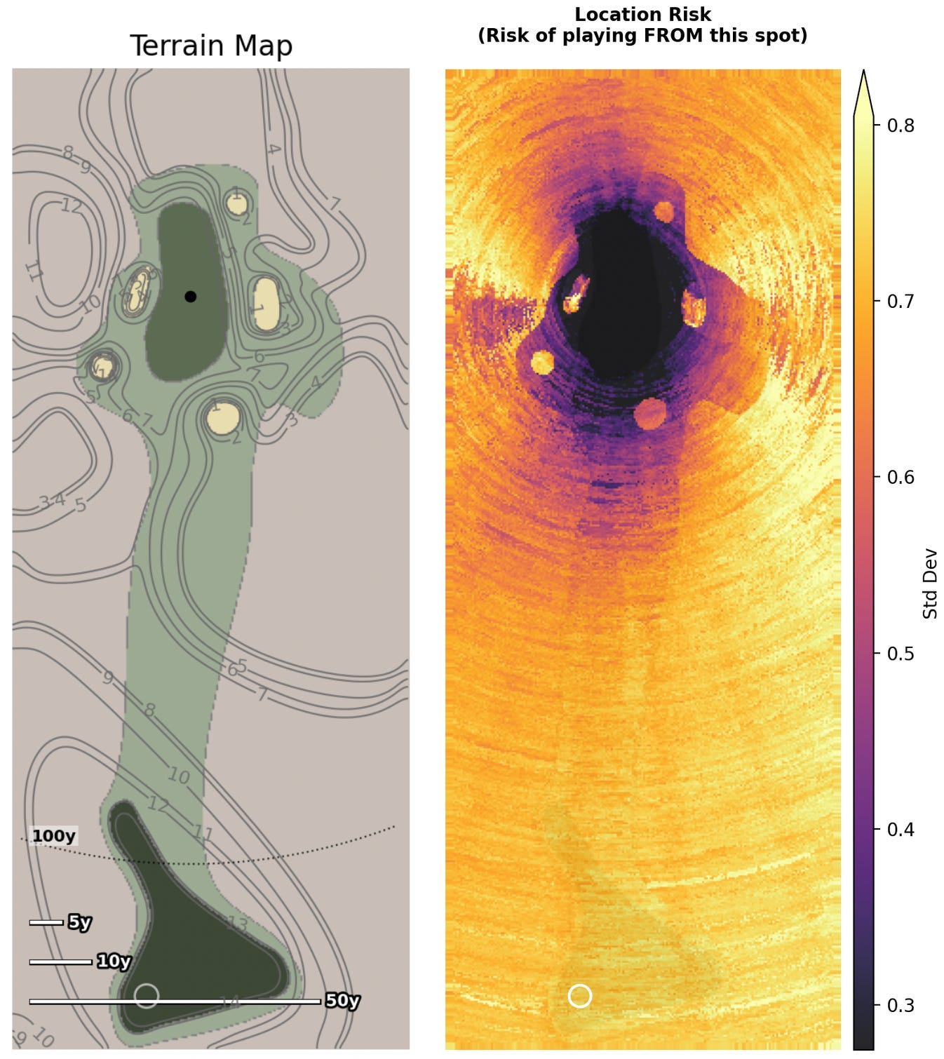
Here we do not see a circular gradient. Just off the green, we see significant high-variance (yellow) areas by the bunkers. We also see low-variance (purple) areas in front of and behind the green.

Normalizing the Scales Shows Extreme Differences

The previous illustrations do not share the same scale because each heatmap is scaled to its own minimum variance and maximum variance. When we set both maps to the same scale, we can see how much more variance Royal Troon actually has:

Standard deviation map of #8 at Sharp Park (left) and #8 at Royal Troon (right) using the same scale to measure variance in strokes to hole.

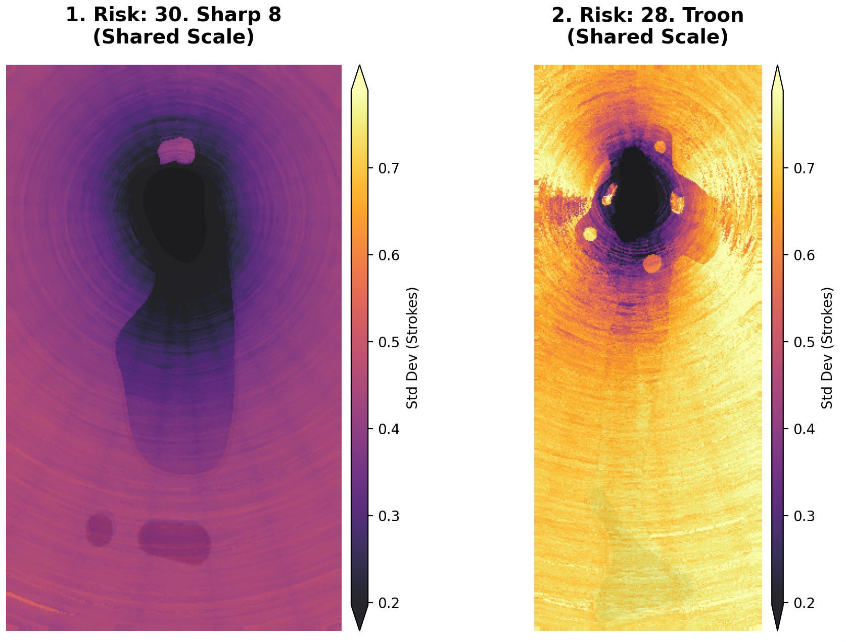
The overall difference in scale here is huge. We should expect the same level of variance from the tee at Sharp Park that we expect from the fringe at Royal Troon.

Variance To vs Variance From

Map #2: Shot Outcome Risk

The standard deviation maps above describe variance from each point on our map. Importantly, though, these maps assume we are hitting an optimal shot. To calculate that optimal shot, however, we iterated through dozens of different shots, and that information will be extremely helpful in illustrating the shot quality/result quality relationship discussed in part one.

So, by way of example, I’ve created an homage to #4 at the Lido, the Channel Hole, but I’ve redesigned the green to dramatically increase the amount of variance.¹ This template has a distinct “island fairway” that lets us reach the green in two shots, but only if we are willing to risk trouble off the tee. The safer option is to bail out to the right, but reaching the green will take three shots. We can see the layout here next to the standard deviation map:

Terrain map and standard deviation map of Channel Hole homage. Clear areas of low variance (purple) can be seen along the safer route (right).

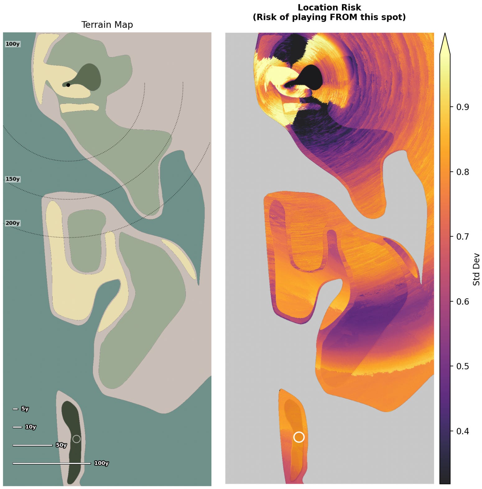
If we’re standing on the tee, the standard deviation map only gives us one pixel of information about our shot. To understand all of our options off the tee, we need to look at variance from the other direction. Here, we know the point where we are hitting our shot from, and we can show the variance involved in playing to every location from that position. The map below is called the “shot outcome risk” map. It shows us the standard deviation of the results of aiming at every possible location from the tee:

Map of standard deviation of results of shot from the tee. Gaussian blur added to results because the Monte Carlo nature of dispersion patterns leads to some pretty irregular results.

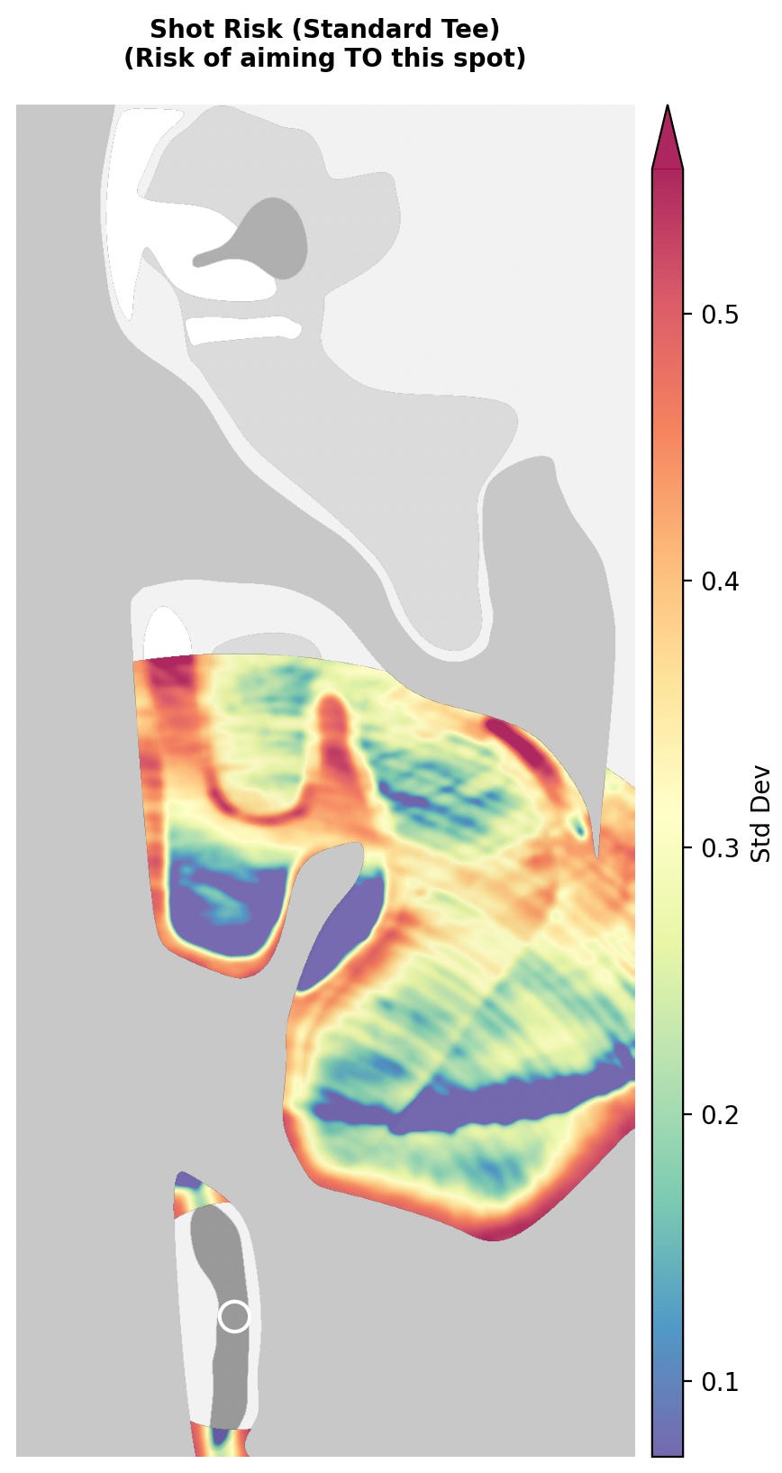
The map shows bright red where the value of shot results is extremely variable. The darkest red areas are near the water hazards and we should expect this. Aiming at the edge of a water hazard will obviously have high variance: about half our misses will end up in the water while the other half will be playable.

One of the major shortcomings of this map, however, is that it doesn’t care whether the results of the shot are good or bad, only that they are consistent. We can see this with the low-variance (dark blue) results in the large bunker on the left side. Yes, hitting a mid-iron into a huge bunker will give consistent results, but they are bad results.

Adding the Risk of the Destination

Map #3: Combined Risk Map

Another shortcoming of the shot outcome map is that it only shows half the variance: the variance to a location. If we add back in the variance from that location, which we have from the standard deviation map, we can see the total variance we take on by playing to each location.

This map shows the combined standard deviations in results from playing TO the target pixel and then the standard deviation of the results of playing FROM that target pixel. The darker locations are by far the most “predictable” locations to play to.

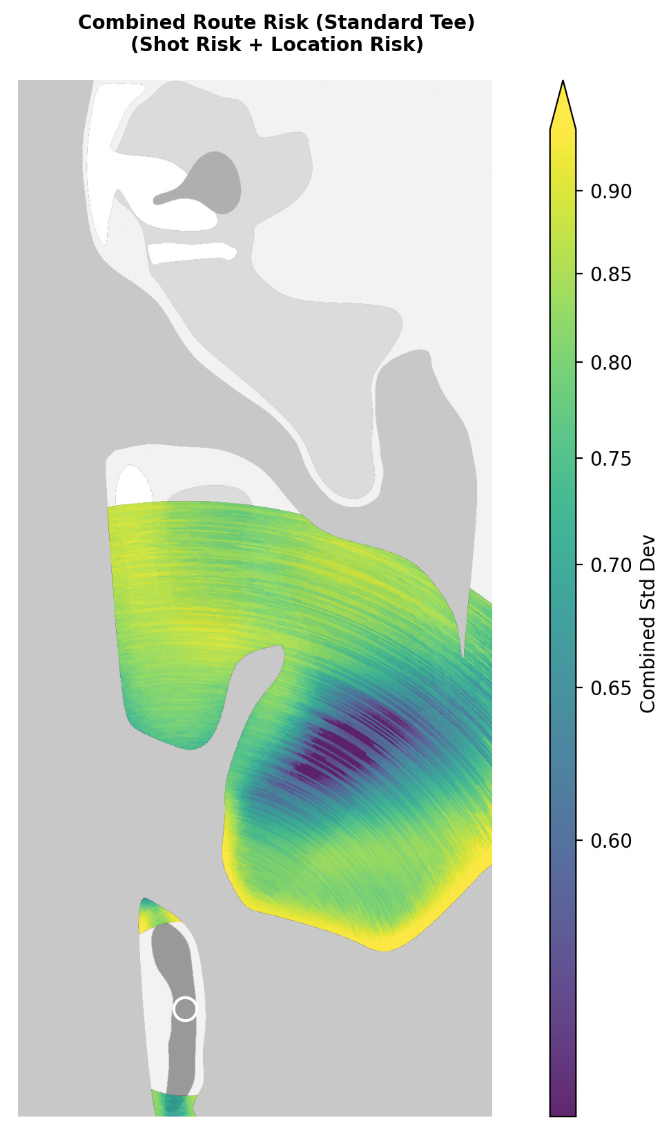
Here, the yellow areas are the most likely to give us an unpredictable path to the hole. The dark blue areas show us where our results will be more consistent on average.

Bailouts and More Philosophy of Golf

The most interesting thing about this map is that, if we look at the fairway areas, it actually shows us bailout zones. The entire function of a “bailout” is to trade expected strokes to hole for lower variance in those strokes-to-hole measurements. Not every golf hole has a bailout area or route, but where they exist, we should expect them to have non-trivially low variance both to and from their location. This map will help us identify them.

Again, however, we’ve been looking at a map that only concerns itself with consistency. If we care about overall scoring results, we’ll need to add expected strokes to hole from each location. We do that in the next map.

Okay, But Where Should I Hit the Ball: Visualizing Strategic Golf

Map #4: Risk-Adjusted Strokes to Hole

We have been slowly building up to a map that illustrates the areas of strategic interest.

This map shows risk-adjusted expected strokes to the hole, given the risks associated with aiming at a location. Assuming we want to avoid risk, we penalize each location’s expected strokes to hole by the standard deviation we should expect TO and FROM that location. Interestingly, it shows no significant difference in playing towards different areas of the fairway.

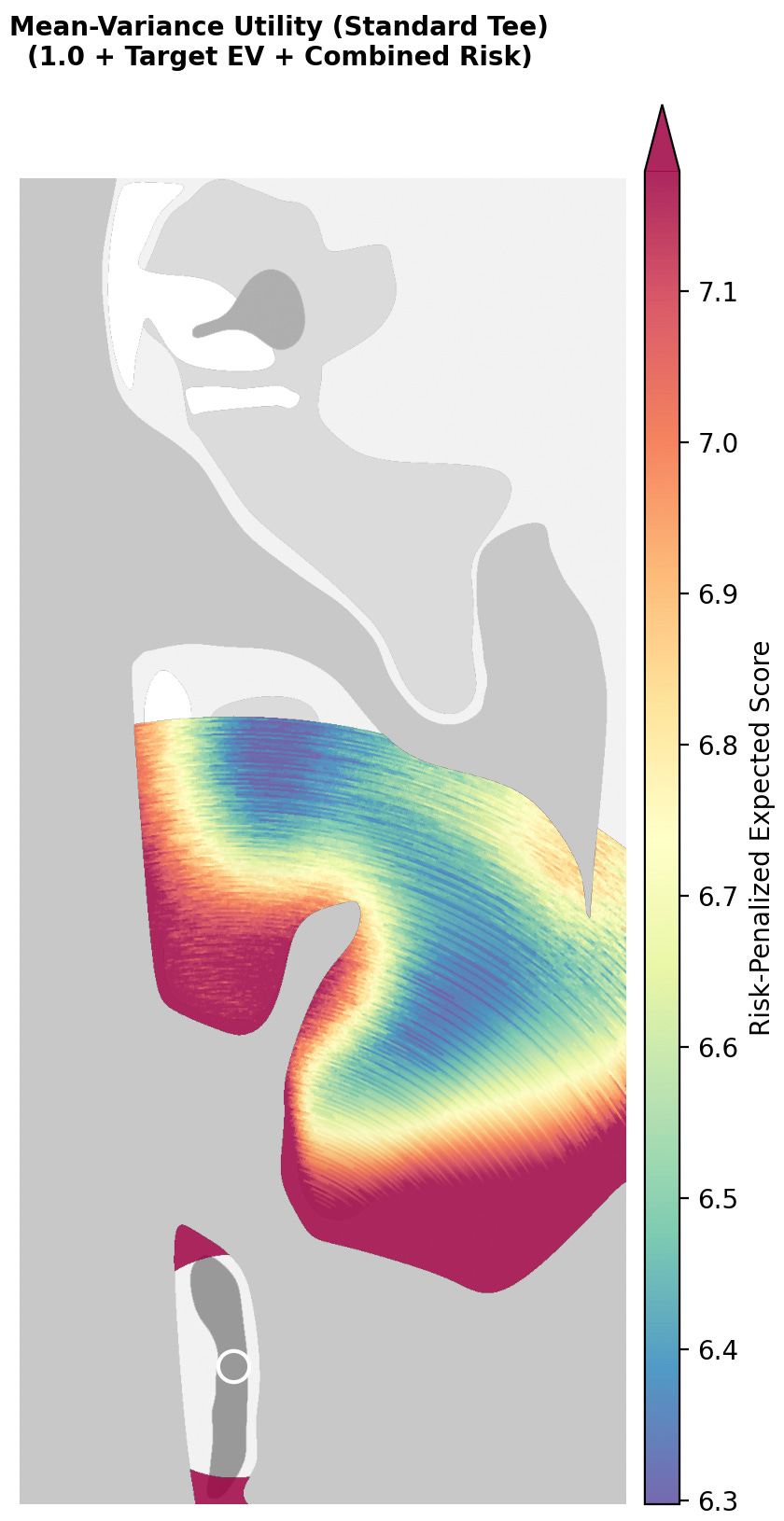
We start with the expected strokes to hole at each location. We then apply a discount rate based on the combined variance to and from each location. This shows us the implied value of expected strokes to hole for every location after accounting for risk.²

It is important to note that this is an inherently risk-averse map. The results skew heavily toward higher scores. This is intentional. While the lowest expected score on this map is 6.3, we don’t actually expect to take 6.3 strokes from those locations. We include a variance penalty at each location, and that penalty shows us which areas are worth that risk.

What we are left with is a map that shows areas of genuine strategic interest. It can’t tell us where to play, but it does highlight the areas where tradeoffs are optimal. I specifically chose this hole design because it allows two clear options for the player. We see that the island fairway and bailout fairway are both strategically interesting. At the same time, we also see that an aggressive line to the bailout fairway is slightly less optimal. Importantly, though, from a design perspective, there are multiple interesting parts of the fairway to aim for.

This hole was designed for strategic optionality, but I want to illustrate risk-adjusted strokes to hole on another design to show what other strategies look like.

Options vs Optimals: Press Your Luck at Woking

If we apply this mapping to #4 at Woking, a different pattern emerges.

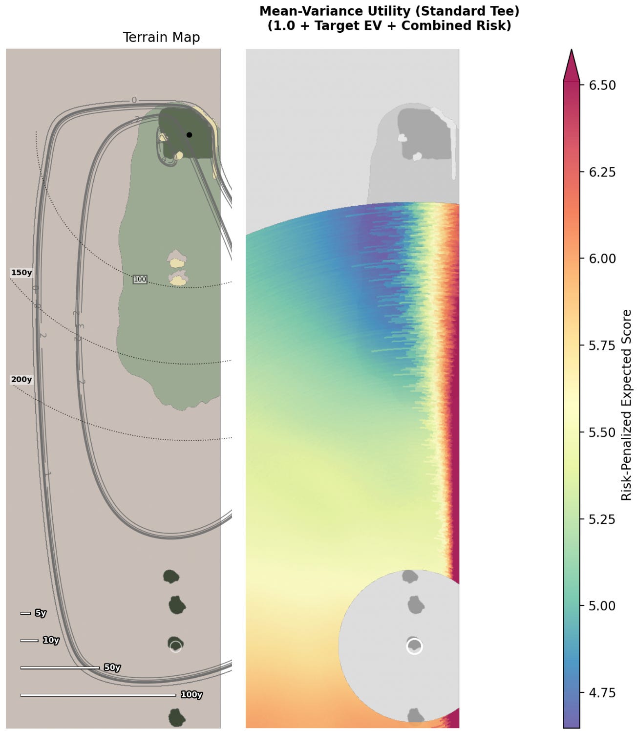
Instead of identifiable zones of interest, we see a pattern where shots become more optimal as the player aims closer to the center of the fairway. However, there is a point after which an aggressive line suddenly leads to terrible results when adjusted for risk. Typically, the sensible play here is to the left side of the fairway; anything else is sub-optimal.³ This is a very clear “press your luck” strategy where players want to take on just enough risk without overdoing it.

This kind of strategy is more narrow. At Woking, there is an optimal place for the risk-averse player, and finding that shot is the goal. At the Lido, by contrast, we have two very different options to choose from. These two holes contrast different kinds of strategy, but they both show up clearly when illustrated as risk-adjusted strokes to hole.

This is a point I want to stress: strategy is not some knob we turn up and down. There are different kinds of strategies, and they can be orthogonal to each other. Importantly, though, we can illustrate these strategic features with risk-adjusted strokes to hole. Players can use this tool to find optimal ways to play a golf hole. Architects can use it to communicate strategic designs to clients and club members.

I would be excited to work with anyone interested in applying these design principles. Please reach out if you want to work with me.

More to Come…

Here, we’ve finished the heavy math and looked at the best ways I’ve found to illustrate variance. In the third part, I’ll be exploring one of the biggest philosophical arguments in golf design: what we mean by “good shots” and “bad shots.” I hope everything has been clear so far. Let me know if you have any questions and I will try to publish part three soon.

1. I’ve changed the Channel Hole homage in a few ways. First, I’ve mirrored the hole. Next, the green is insanely high variance. The pin sits on a narrow peninsula section of the green, surrounded by sand. Finally, the landing zone short of the green is significantly wider than the real version.

2. Now, there are two important caveats here:

1. This map is still player-specific. When looking at these maps, we are only seeing areas of strategic interest for the player with the distance/dispersion that we’ve used here: in this case, a 15 HCP generated with my golf shot dispersion simulator. The strategic interest will be different for different players. A professional will interact with the strategic elements of a golf hole very differently than a bogey golfer will.

2. The discount rate we use to penalize certain areas of the fairway is variable. I’ve chosen raw combined standard deviation as a simple discount rate, but players who are more risk-seeking (e.g. in a Stableford format) or more risk-averse (trying to maintain a lead) will want to adjust their discount rate accordingly. The map should appear mostly the same with different discount rates, though the contours could change at the margins.

Note: I use the mean of variances to combine the two standard deviation metrics. We cannot add our standard deviations together directly.

3. I would note again that “optimal” strategies here assume a specific risk tolerance. A more risk-seeking player will likely be more willing to take on the right side of the fairway, and we can adjust our variance discount rate to suit that.